A web application designed to enable easy programming and creation of Light Program Files (LPFs) for use in Tabor Lab optogenetic hardware. It uses HTML5 and JavaScript to acquire desired light function parameters, perform intensity & staggered-start calculations, and finally deliver output files to the user, all in the browser.
Details about Iris and the optogenetic hardware it supports have been published in Scientific Reports.
Iris is designed to be a flexible interface for the Tabor Lab standardized optogenetic hardware platform. It is able to:
Note that for advanced users, there is also a standalone Python library that can convert more complex and arbitrary light programs into device-readable LPF files; however Iris should be sufficient for all normal use cases.
A variety of devices are supported in addition to those detailed in our publication, though the most common selection will be the 24-well plate device (LPA). This will automatically configure Iris to have the correct number of wells and correct LED wavelengths for simulation later. If you have a custom device running appropriate firmware, then you can use the Custom Configuration, which will prompt you to enter the number of rows and columns in your custom device, as well as the number of LEDs in each well and their wavelengths in the section that appears.
There are three input styles that can be used to create light programs: Steady State, Simple Dynamic, and Advanced Dynamic. Each will significantly change the programming layout for creating the corresponding programs, as described below:
Some parameters apply to the entire experiment: the total program time duration (in minutes), whether wells should be programmed column-wise or row-wise, whether the well positions should be randomized, and whether the LEDs should all be turned off at the end of the experiment (check boxes). The Program Duration should include all phases of the experiment, including any dark or preconditioning phases, which will be specified later. If you choose to randomize the well positions (highly recommended), the generated randomization matrix will be provided when you download the LPF so that you can descramble the data during analysis. We recommend turning off the LEDs at the end of the experiment, since this serves as a convenient indicator that the program has run its complete course.
Note: These parameters do not apply to the Steady-State input style. Only the Program Duration applies to the Simple Dyanamic input style.
If there are wells in the device that should not be programmed, these can be eliminated from Iris' calculations by right clicking them in the simulation panel. They will be marked by a large X and will be skipped as Iris fills wells. These wells will be programmed to keep their LEDs off for the entire length of the experiment. The selection of eliminated wells may be updated at any point during the Iris session.
In the Advanced Dynamic input style, Experiments define groups of wells in the plate device that are related, typically because they are all time points or measurements of the same dynamic experiment (i.e. all wells are receiving versions of the same input signal with staggered start times). An Experiment can utilize any number of wells in the plate, and the number used by a particular Experiment will automatically be updated as inputs are entered. All Experiments (and Waveforms) can be minimized at any time during input to make room for additional input elements by clicking the chevron to the left of the Experiment header.
Note: All the parameters below are set automatically in the Steady State and Simple Dynamic input styles.
In an Advanced Dynamic program, Iris can automatically generate a set of evenly-spaced time points or use a custom set (to focus data on early-time responses, for example). For generated time points, enter the number of desired time points and the delay (in minutes) until the first time point, if any. For custom time points, simply paste a list of comma-separated time points into the array (all units in minutes). Steady-state experiments should use the default value of 1 for the number of time points.
Enter the number of experimental replicates of this experiment. The number of wells specified by the Experiment's Waveform inputs will be replicated across the plate Replicates number of times (i.e. Replicates = 1 indicates that no additional wells will be used). Note that this will very quickly consume available wells.
Several waveforms (Constant and Step) are able to take multiple inputs, which are then automatically expanded by Iris into a number of wells. The default behavior when more than one of these waveforms is entered in a particular Experiment is for every combination of the intensities specified to be created. For example, if Constant Waveform 1 indicates 2 intensities for the red LED (123, 234 GS) and Constant Waveform 2 indicates 2 intensities for the green LED (1234, 2345 GS), then 4 wells will be used: (123, 1234), (123, 2345), (234, 1234), and (234, 2345) for the R/G LED intensities, respectively. This makes it very easy to specify a series of arbitrary intensities for one LED, while keeping another LED constant in all wells: Waveform 1 would indicate the arbitrary intensities, and Waveform 2 would only need a single intensity, which would then be applied to the arbitrary wells. We refer to this result as a Combination of waveforms.
Alternatively, some experiments require arbitrarily chosen LED intensities in more than one channel. Instead of creating a separate Experiment for each set of intensities in a particular well, Iris can be programmed to integrate multiple Constant waveforms differently: Addition. Rather than creating every combination of input intensities, Iris will associate lists of intensities in an element-wise fashion. For example, in the same scenario as above, the result will be only 2 wells: (123, 1234) and (234, 2345). Note that for Addition, the lengths of the lists of intensities must be equal. Additionally, a Constant Waveform cannot be Added to any other type of (dynamic) waveform -- when a dynamic waveform is added to the Experiment, Iris automatically defaults to the above Combination behavior.
For Dynamic input styles, the four icons represent the four fundamental waveform inputs programmed into Iris: constant, step change, sinusoid, and arbitrary, which can be added to the Experiment by clicking the corresponding icons. Each Waveform represents a light input applied to the desired wells in a particular LED channel. Importantly, waveforms cannot be composed - that is, multiple waveforms cannot be applied to the same LED in the same well. More complex inputs (e.g. a series of step inputs) should be entered using the (more efficient) Arbitrary Waveform. Note that all light intensities (amplitudes) are given in hardware greyscale units (GS), which must be in the range \([0,4095]\). Also note that if multiple intensities are given to the Constant or Step Waveforms, each intensity will be separately applied to every other waveform in the experiment, since multiple intensities of a single LED cannot be applied to the same well. In other words, every possible combination of Waveforms is programmed. For example, if 2 intensities are entered in a Step Waveform, and the Experiment specifies 10 samples ("time points") and 1 replicate, the Experiment will use 20 wells in the plate.
\[f(t) = c\] Constant inputs are used to apply competing amounts of deactivating light and to measure the steady-state dose response function. Obviously, they only have a single input parameter.
\[f(t) =\begin{cases}I_o & t < t_s\\I_f & t \geq t_s\end{cases}\] Step inputs are used for dynamic characterization and have 3 parameters:
\[f(t) = a * \sin \left(\frac{2\pi \left(t - \phi\right)}{T}\right) + c\] Sinusoidal inputs are an alternative input signal for dynamic characterization and have 4 parameters:
\[f(t) = \sum_{i=0}^n a_i H(t-\tau_i)\] Arbitrary Waveforms allow input of any more complex function as a series of light intensities (\(a_i\)) and corresponding times at which the LED will switch to that intensity (\(\tau_i\)). These are entered as a list of values in the Excel-like table under their respective headings. The switch times are the time since the beginning of the experiment (not related to time points), in minutes. The light intensities are in greyscale (GS) units. Because the smallest time resolution for the resulting LPF file is 1 sec, this is also the smallest valid time step for arbitrary inputs.
To load a simulation of the specified light program, first ensure that no input fields have been marked as invalid. A tooltip will appear on mouse-over to indicate the relevant error for a particular field, if it is invalid. (Errors in Arbitrary or Steady State input tables are highlighted by red cells.) If the inputs for each Experiment are valid, Iris will automatically load a hardware simulation in the right hand panel. This simulation has two aspects: Plate View, which is an overview of LED intensity over time for the entire plate; and Well View, which displays a light time-course plot for all LEDs in a particular well.
The default view is Plate View, which shows an overview of the entire plate device. Using the drop-down menu in the navigation bar at the top, the display can be limited from showing all (illuminated) LEDs to only particular LEDs. Clicking on a well in the plate visualization will select that well, updating the position and well number in the nav bar. The up, down, left, and right arrow keys can also be used to change the selected well. Clicking the play button will begin the hardware simulation, and will show the response of the plate device to the generated light program over time. The Speed slider bar will decrease or increase the simulation playback speed.
To get more detail about a particular well, simply click the well in Plate View and then click Well View in the nav bar. Well View plots the LED intensity for all LEDs in a well as a function of time. Click and drag horizontally in the plot area to zoom in on that region of the plot. Notice that, again, the smallest time resolution for the program is 1 sec, which will cause some apparent aliasing at small timescales. To remove the plot for an LED, simply click its entry in the legend. A floating tooltip indicates the LED intensities corresponding to the time currently under the mouse cursor. The arrow keys will still change the selected well and can be used to rapidly move through adjacent wells' Well Views.
If everything looks good, then initiate the download of the generated files by clicking the Download button at the bottom of the inputs. The zipped folder includes the following files:
It is crucial that these files not get separated from each other. Without an IRS file, it is impossible (using Iris) to determine what program a particular LPF file encodes, and the hardware does not allow this file to be renamed! That said, it is possible to parse LPF files using scripts (see to the standalone Python code.) Instead, however, we recommend simply keeping these files together and loading up a IRS file to reload exactly the Iris session that produced the corresponding LPF.
Furthermore, loss of the randomization matrix will make the data impossible to analyze. There is no way to extract the randomization matrix from the LPF program, though it can be recovered (re-downloaded) from the Iris session savefile.
If the corresponding box is checked, Iris will randomize the positions of all wells in the plate. The Randomization Matrix (RM) can be accessed the CSV file of the same name in the downloaded zip folder. In plain language, the values in the RM represent the true (descrabled) positions in the plate of the data for a particular well. For example, if the first value (index 0) in the RM is 11, then the data from the first well in the plate (index 0) should be moved to the well with index 11 (well number 12). Be careful not to do this backwards!
To perform this de-randomization in Excel, simply add a new column to the randomization matrix CSV containing data values from each well (match to Well Number / Plate Coordinates). Next, sort the CSV data by the Randomization Matrix column. The data values will now be de-randomized and can be plotted against the Time Points column.
Some example Python code to perform this de-randomization:
    rand_mat = [4, 0, 1, 3, 2] # Example Randomization Matrix
    measured_data = [567, 123, 234, 456, 345] # Toy measured data for wells: 0, 1, 2, 3, 4
    descrambled_data = [0, 0, 0, 0, 0] # Empty; will hold the descrambled data values
    total_well_num = 5
    for i in range(total_well_num):
        descrambled_data[rand_mat[i]] = measured_data[i]
    print descrambled_data
    ## Prints: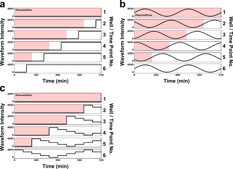
## [123, 234, 345, 456, 567]In order to perform dynamic light experiments, the input signal applied to each well in an experiment is staggered such that at the end of the program, that well will end at the desired time point in the waveform, as previously validated using our test-tube based Light Tube Array (Olson et al., Nature Methods, 2014). The time difference created by staggering the input is filled by exposing the well to the Preconditioning light condition (table below) for all times before the time-shifted waveform begins (red overlay). For example, the t=560min time point (Well 5, below) in a 720min experiment will experience the Preconditioning light condition for 160min, and then begin the staggered program. It will experience the first 560min of the waveforms in each of its LED channels, at which point the experiment will end. This procedure is repeated for all wells (time points) in an experiment, and can be visualized in Iris under Well View.
More specifically, the Preconditioning light input for each function is as follows:
| Input Waveform | Precondition Value |
|---|---|
| Constant | N/A |
| Step | Input intensity before step (i.e. the step offset, \(c\)) |
| Sine | Because sines are periodic, no precondition state is necessary; the function is simply phase shifted by the appropriate amount. |
| Arbitrary | The precondition light intensity for Arbitrary waveforms is set by the user in the waveform input spreadsheet. |
The LPF binary should not need to be examined directly during the standard workflow; however, its format is detailed below should it be necessary:
The LPF file has a header segment encoded by 32-bit (4-byte) ints:
| Bytes | Variable Name | Precondition Value |
|---|---|---|
| 0-3 | FILE_VERSION | LPF version number, currently 1 |
| 4-7 | NUMBER_CHANNELS | number of channels -- Note: This is the total number of LED channels (e.g. 2*24 = 48), not per well |
| 8-11 | STEP_SIZE | time step size, in ms (default: 1000ms to limit total program file size) |
| 12-15 | NUMBER_STEPS | number of time points (total program time / STEP_SIZE + 1) |
| 16-31 | --empty-- | Reserved space for future header fields; all set to 0 |
| >= 16 | n/a | intensity values of each channel per time point. For each value, two bytes will be used as a long 16-bit int |
LED intensity values are listed for a single time point in a depth-first manner (i.e. all LEDs for a particular well, then proceeding to the next well), moving top-to-bottom, and left-to-right across the plate device. The LED order is a hard-coded parameter for each device, and is dependent on the particular configuration of the PCB. After the final LED intensity of the final well, the LPF continues with the next time step.
Because of the above structure, specifically that every time step is encoded explicitly, and that each is encoded using a 16-bit (2 byte) integer, file sizes can quickly become very large at small time steps or long program lengths. To keep things reasonable, we limit time steps to 1 sec, minimum. The time step is automatically increased to 10s for LPF programs longer than 12hr.
The following packages and utilities were used in the creation of Iris:
The standalone Python LPF Encoder script uses Numpy and was made using iPython Notebook.
Iris should be fully functional on all up-to-date versions of: Chrome & Safari. The LPF file size limit, set by the FileSaver.js package, is limited by Chrome, which only allows files smaller than 500MB.
Iris should be accessable online, but it can be run offline as well. To do so, follow these steps:
python -m SimpleHTTPServer to begin the HTTP server.http://localhost:XXXX, where XXXX is the port number the HTTP server is using.Requires Numpy.
Occasionally, users comfortable with coding may want to quickly create algorithmic LPF files based on custom code outside of Iris. To facilitate this, a simple python script has been added that can do just this. It will (hopefully) be maintained in parallel with any changes to the header information & LPF format in the main Iris code.
To create an LPF in this way, users will have to ensure that their data is in a Numpy matrix with the correct dimensionality (indices refer to: [Time][wellNumber][channelNum]). The user is entirely responsible for ensuring that their matrix matches the device they have chosen to use. The second input parameter is a dictionary of device parameters for the header of the LPF: 'channelNum' is the TOTAL number of channels (channels per well * number of wells); 'timeStep' is the time step in ms; 'numSteps' is the total number of time steps in the LPF. Finally, the given file name is the complete (relative) path to the desired file location AND the desired file name, including suffix (.lpf).
The easiest way to submit a bug report or pull request is to email . Alternatively, Iris is an open-source project; therefore, the GitHub repository housing all Iris code is available for contributions. Any bugs identified can be logged in the project's Issues section, and proposed improvements can be submitted as Pull Requests.
Copyright (c) 2015, Felix Ekness, Lucas Hartsough, Brian Landry. All rights reserved.
Redistribution and use in source and binary forms, with or without modification, are permitted provided that the following conditions are met:
THIS SOFTWARE IS PROVIDED BY THE COPYRIGHT HOLDERS AND CONTRIBUTORS "AS IS" AND ANY EXPRESS OR IMPLIED WARRANTIES, INCLUDING, BUT NOT LIMITED TO, THE IMPLIED WARRANTIES OF MERCHANTABILITY AND FITNESS FOR A PARTICULAR PURPOSE ARE DISCLAIMED. IN NO EVENT SHALL THE COPYRIGHT HOLDER OR CONTRIBUTORS BE LIABLE FOR ANY DIRECT, INDIRECT, INCIDENTAL, SPECIAL, EXEMPLARY, OR CONSEQUENTIAL DAMAGES (INCLUDING, BUT NOT LIMITED TO, PROCUREMENT OF SUBSTITUTE GOODS OR SERVICES; LOSS OF USE, DATA, OR PROFITS; OR BUSINESS INTERRUPTION) HOWEVER CAUSED AND ON ANY THEORY OF LIABILITY, WHETHER IN CONTRACT, STRICT LIABILITY, OR TORT (INCLUDING NEGLIGENCE OR OTHERWISE) ARISING IN ANY WAY OUT OF THE USE OF THIS SOFTWARE, EVEN IF ADVISED OF THE POSSIBILITY OF SUCH DAMAGE.